Practice Final #1
Full CourseExam Settings
Mixed Content
Mixed ContentExercise Tags
Tag:
Use the tag filtering feature on the course homepage to find all exercises with this tag.
Prerequisites for this Exercise
No prerequisite skills selected yet.
Unlock Premium Content
Get instant access to detailed walkthroughs, step-by-step explanations, and exclusive learning materials.
For to be differentiable everywhere, it must first be continuous everywhere. This means the two pieces of the function must meet at the point where their definitions change, which is at . The value of the top function at must equal the value of the bottom function at .
Evaluate the top part of the function at :
Now, set the bottom part of the function equal to this value at :
For to be differentiable at , the slopes of the two pieces must be equal at that point. We find the slope by taking the derivative of each part of the function.
Take the derivative of the top part, :
Evaluate this derivative at :
Take the derivative of the bottom part, :
For differentiability, the derivatives must be equal at :
For a piecewise function to be differentiable at the point where its definition changes, both the function values and their derivatives must be equal at that point.
Now we have a system of two equations with two unknowns:
1.
2.
Substitute from Equation 2 into Equation 1:
Thus, the values for and that make the function differentiable everywhere are and .
The final solution is:
Unlock Premium Content
Get instant access to detailed solutions, step-by-step explanations, and exclusive learning materials.
Exercise Tags
Tag:
Use the tag filtering feature on the course homepage to find all exercises with this tag.
Prerequisites for this Exercise
No prerequisite skills selected yet.
Unlock Premium Content
Get instant access to detailed walkthroughs, step-by-step explanations, and exclusive learning materials.
Unlock Premium Content
Get instant access to detailed solutions, step-by-step explanations, and exclusive learning materials.
Sub-questions:
Exercise Tags
Tag:
Use the tag filtering feature on the course homepage to find all exercises with this tag.
Prerequisites for this Exercise
No prerequisite skills selected yet.
Unlock Premium Content
Get instant access to detailed walkthroughs, step-by-step explanations, and exclusive learning materials.
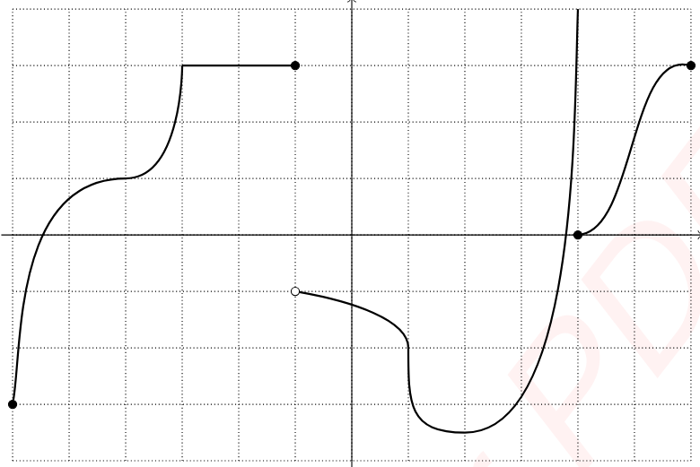
The first place to look is where . But this is just a derivative of 0, so that's totally fine.
Next we look at . This is a 'cusp' since it's a 'sharp turn' or 'corner'.
Any 'sharp turn' in a function are called a cusp and the derivative does not exist there.
So at we know the derivative does not exist.
Next we look at . Since the function is not even continuous there, we therefore also know that the function is not differentiable there.
So we add to our list.
The next point in question is when . Since it looks like the slope is completely vertical at , that makes the slope essentially infinite. That means the derivative does not exist there!
The derivative does not exist for any value where the function is totally vertical.
Moving on to the next point in question would be where . The function is not continuous there so therefore it is also not differentiable.
Unlock Premium Content
Get instant access to detailed solutions, step-by-step explanations, and exclusive learning materials.
which is the same as:
Exercise Tags
Tag:
Use the tag filtering feature on the course homepage to find all exercises with this tag.
Prerequisites for this Exercise
No prerequisite skills selected yet.
Unlock Premium Content
Get instant access to detailed walkthroughs, step-by-step explanations, and exclusive learning materials.
From the graph we can see the slope is negative starting when and continues to be negative until .
There are two important exceptions when and when . The derivative does not exist at either of those points, so we can't include them in our final answer. Let's explain this:
When we have no left side limit, so the derivative does not exist.
When the derivative does not exist because the left hand limit and right hand limit both approach infinity.
So for our final answer we have only:
Unlock Premium Content
Get instant access to detailed solutions, step-by-step explanations, and exclusive learning materials.
Another way to say it is this:
Exercise Tags
Tag:
Use the tag filtering feature on the course homepage to find all exercises with this tag.
Prerequisites for this Exercise
No prerequisite skills selected yet.
Unlock Premium Content
Get instant access to detailed walkthroughs, step-by-step explanations, and exclusive learning materials.
NOTE: These points do not necessarily indicate an inflection point! For instance take the parabola when .
From the graph we can see an inflection point at together with a tangent line of finite slope (in this case the slope is 0), so the second derivative must be 0 there.
We also definitively have an inflection point when since the graph changes from concave up to concave down together with a tangent line. So for sure we have here at too.
We can't really tell what's happening when , but for this case the answer key will almost certainly not include this point. It's a local min which can indeed sometimes have (an example was given earlier with at ).
Careful with . Since the first derivative doesn't exist there, the second derivative can't exist either. So we have only at and .
Final solution is:
or just :
Unlock Premium Content
Get instant access to detailed solutions, step-by-step explanations, and exclusive learning materials.
or just :
Exercise Tags
Tag:
Use the tag filtering feature on the course homepage to find all exercises with this tag.
Prerequisites for this Exercise
No prerequisite skills selected yet.
Unlock Premium Content
Get instant access to detailed walkthroughs, step-by-step explanations, and exclusive learning materials.
We can see a small concave up segment from when is between and .
Then it looks like another small segment when is between 1 and 4.
Then finally there is a small interval where is concave up right near then end when is between 4 and 5.
Note that x=4 is not included.
Unlock Premium Content
Get instant access to detailed solutions, step-by-step explanations, and exclusive learning materials.
Exercise Tags
Tag:
Use the tag filtering feature on the course homepage to find all exercises with this tag.
Prerequisites for this Exercise
No prerequisite skills selected yet.
Unlock Premium Content
Get instant access to detailed walkthroughs, step-by-step explanations, and exclusive learning materials.
Unlock Premium Content
Get instant access to detailed solutions, step-by-step explanations, and exclusive learning materials.
Exercise Tags
Tag:
Use the tag filtering feature on the course homepage to find all exercises with this tag.
Prerequisites for this Exercise
No prerequisite skills selected yet.
Unlock Premium Content
Get instant access to detailed walkthroughs, step-by-step explanations, and exclusive learning materials.
The derivative of with respect to is:
We are differentiating , so we need to apply the chain rule because we have a function inside another function (i.e., inside ).
According to the chain rule, if you have a composite function , its derivative is:
Here, , so:
The derivative of with respect to is:
Now, substitute the derivative of into the expression:
Thus, the derivative of is:
Unlock Premium Content
Get instant access to detailed solutions, step-by-step explanations, and exclusive learning materials.
Exercise Tags
Tag:
Use the tag filtering feature on the course homepage to find all exercises with this tag.
Prerequisites for this Exercise
No prerequisite skills selected yet.
Unlock Premium Content
Get instant access to detailed walkthroughs, step-by-step explanations, and exclusive learning materials.
To find the derivative of:
we will apply the quotient rule.
The quotient rule states that for a function of the form , the derivative is:
Here, and .
We need the derivatives of both and :
- The derivative of is:
- The derivative of is:
Substitute the functions and their derivatives into the quotient rule:
Simplify the numerator:
Using the identity , the expression becomes:
Using the identity is a key trick that simplifies many trigonometric expressions involving inverse trigonometric functions.
Thus, the derivative of is:
Unlock Premium Content
Get instant access to detailed solutions, step-by-step explanations, and exclusive learning materials.
Exercise Tags
Tag:
Use the tag filtering feature on the course homepage to find all exercises with this tag.
Prerequisites for this Exercise
No prerequisite skills selected yet.
Unlock Premium Content
Get instant access to detailed walkthroughs, step-by-step explanations, and exclusive learning materials.
The expression is , which contains two terms:
1. The first term is . This is an exponential function where the base is and the exponent is .
2. The second term is . Here, the base is , and the exponent is .
For differentiation, we need to treat each term carefully using rules such as the chain rule and logarithmic differentiation.
The first term is . Applying the chain rule:
Now, differentiate . Since is a constant, the derivative of is:
So, the derivative of the first term becomes:
The second term is . To differentiate this, we use logarithmic differentiation. Let:
Now differentiate both sides implicitly:
Solving for :
Now, combine the derivatives of both terms:
Thus, the derivative of the expression is:
This question tests your understanding of **differentiation rules for composite and complex functions**. The goal is to assess whether you can correctly apply the chain rule for exponential functions and **logarithmic differentiation** for functions where both the base and exponent are dependent on .
By mastering this problem, you are developing the ability to handle advanced differentiation tasks involving multiple rules, which is essential for success in calculus.
Unlock Premium Content
Get instant access to detailed solutions, step-by-step explanations, and exclusive learning materials.
Exercise Tags
Tag:
Use the tag filtering feature on the course homepage to find all exercises with this tag.
Prerequisites for this Exercise
No prerequisite skills selected yet.
Unlock Premium Content
Get instant access to detailed walkthroughs, step-by-step explanations, and exclusive learning materials.
We are tasked with finding the limit:
This expression involves two exponential terms: and .
Let’s analyze the behavior of both terms:
1. The term : As , the exponent grows large, making very large.
2. The term : As , the exponent grows even faster, making grow much larger than .
This results in an indeterminate form: .
To simplify the expression, we take the natural logarithm. Define:
Taking the natural logarithm of both sides:
Simplifying further:
This limit involves terms that grow at different rates as , making it useful to find a common denominator to better analyze their behavior.
The least common denominator between and is . Rewrite each term with this common denominator:
Now, combine the terms:
As , the term vanishes, leaving:
Since the numerator is a negative constant and the denominator grows large, the limit is:
Since:
The limit is:
The professor likely asked this question to assess your understanding of indeterminate forms and your ability to apply logarithmic transformations effectively. This problem reinforces the idea that in calculus, growth rates of different functions (like exponential terms) are crucial for evaluating limits.
Unlock Premium Content
Get instant access to detailed solutions, step-by-step explanations, and exclusive learning materials.
Exercise Tags
Tag:
Use the tag filtering feature on the course homepage to find all exercises with this tag.
Prerequisites for this Exercise
No prerequisite skills selected yet.
Unlock Premium Content
Get instant access to detailed walkthroughs, step-by-step explanations, and exclusive learning materials.
We are tasked with solving:
As , both and approach 0. This results in the indeterminate form , making this a case for applying L'Hopital's Rule.
Remember, L'Hopital's Rule applies when the limit results in either or .
We apply L'Hopital's Rule by differentiating the numerator and denominator separately.
1. **Differentiate the numerator** :
- The derivative of is , and the derivative of is 1. Thus:
2. **Differentiate the denominator** :
- The derivative of is , and the derivative of is 1. Thus:
Now, the limit becomes:
Evaluating both the numerator and the denominator at :
- , so .
- , so .
We encounter the indeterminate form again, so we apply L'Hopital's Rule a second time.
Applying L'Hopital's Rule multiple times is perfectly valid when necessary.
1. **Differentiate the numerator** :
- The derivative of is .
2. **Differentiate the denominator** :
- The derivative of is .
Now, the limit becomes:
For small , we use the small-angle approximations and . Thus:
For very small values of , and behave similarly, leading to:
Thus, the value of the limit is:
This problem tests your ability to use L'Hopital's Rule effectively and repeatedly. It emphasizes the importance of knowing small-angle approximations for functions like and . Additionally, the exercise aims to develop an intuition for recognizing when two functions behave similarly for small inputs.
Unlock Premium Content
Get instant access to detailed solutions, step-by-step explanations, and exclusive learning materials.
Exercise Tags
Tag:
Use the tag filtering feature on the course homepage to find all exercises with this tag.
Prerequisites for this Exercise
No prerequisite skills selected yet.
Unlock Premium Content
Get instant access to detailed walkthroughs, step-by-step explanations, and exclusive learning materials.
We are tasked with solving:
As approaches , both and tend to infinity, creating the indeterminate form . To properly evaluate this limit, we need to manipulate the expression into a form suitable for limit evaluation.
When dealing with indeterminate forms like , it’s helpful to simplify the terms into a single fraction.
We express and using sine and cosine functions:
Now, the limit becomes:
We can factor out from both terms:
As approaches :
- .
- .
Thus, the expression approaches the indeterminate form , making it suitable for applying L'Hopital's Rule.
We differentiate the numerator and the denominator separately:
1. **Differentiate the numerator** :
- The derivative of is 0, and the derivative of is . Thus:
2. **Differentiate the denominator** :
- The derivative of is . Thus:
Now, the limit becomes:
As :
- .
- .
Thus, the limit simplifies to:
The value of the limit is:
This problem is designed to test your understanding of **trigonometric identities** and how to handle **indeterminate forms** using L'Hopital's Rule.
Unlock Premium Content
Get instant access to detailed solutions, step-by-step explanations, and exclusive learning materials.
Exercise Tags
Tag:
Use the tag filtering feature on the course homepage to find all exercises with this tag.
Prerequisites for this Exercise
No prerequisite skills selected yet.
Unlock Premium Content
Get instant access to detailed walkthroughs, step-by-step explanations, and exclusive learning materials.
To find the equation of the tangent line to a function at a specific point , we use the **point-slope form** of a line:
Here, , and we need to find the tangent line at .
First, evaluate the function at :
Thus, the point on the curve is .
The derivative of is:
Now, evaluate the derivative at :
Thus, the slope of the tangent line at is .
Remember, the slope of the tangent line is the derivative evaluated at the given point.
We have the slope and the point . Using the point-slope form:
Simplify the equation:
Thus, the equation of the tangent line is:
The equation of the line tangent to at is:
This problem helps you practice finding the **equation of a tangent line** using the **point-slope formula**.
Unlock Premium Content
Get instant access to detailed solutions, step-by-step explanations, and exclusive learning materials.
Sub-questions:
Exercise Tags
Tag:
Use the tag filtering feature on the course homepage to find all exercises with this tag.
Prerequisites for this Exercise
No prerequisite skills selected yet.
Unlock Premium Content
Get instant access to detailed walkthroughs, step-by-step explanations, and exclusive learning materials.
From part (a), the equation of the tangent line to at was:
This equation gives us a linear approximation for around .
Linear approximations are most accurate near the point where the tangent line is calculated. Here, we use the tangent line to estimate .
1. **Substitute into the tangent line equation:**
2. **Simplify the expression:**
We start by rewriting the fractions with a common denominator. The least common denominator of and is 10:
Now simplify:
Thus, the linear approximation for is:
The linear approximation of based on the tangent line at is:
Linear approximations work best for values close to the point of tangency. Here, the approximation is most accurate for near .
Unlock Premium Content
Get instant access to detailed solutions, step-by-step explanations, and exclusive learning materials.
Exercise Tags
Tag:
Use the tag filtering feature on the course homepage to find all exercises with this tag.
Prerequisites for this Exercise
No prerequisite skills selected yet.
Unlock Premium Content
Get instant access to detailed walkthroughs, step-by-step explanations, and exclusive learning materials.
The volume of a right circular cylinder with height and radius is given by the formula:
We are asked to find how fast the volume is changing with respect to time, i.e., , at a specific moment when:
- and increasing at a rate of ,
- and decreasing at a rate of .
To find how fast the volume is changing, we differentiate with respect to time using the product rule. The radius and height are both functions of time, so we apply the chain rule:
This equation accounts for the rates of change of both the radius and the height.
We are given the following information at the instant of interest:
- ,
- ,
- ,
- .
Substitute these values into the differentiated volume equation:
Now, simplify each term in the expression:
Thus, the rate of change of the volume is:
The volume of the cylinder is increasing at a rate of:
Use the product rule when differentiating expressions with multiple variables that change with time.
Unlock Premium Content
Get instant access to detailed solutions, step-by-step explanations, and exclusive learning materials.
Exercise Tags
Tag:
Use the tag filtering feature on the course homepage to find all exercises with this tag.
Prerequisites for this Exercise
No prerequisite skills selected yet.
Unlock Premium Content
Get instant access to detailed walkthroughs, step-by-step explanations, and exclusive learning materials.
Unlock Premium Content
Get instant access to detailed solutions, step-by-step explanations, and exclusive learning materials.
Sub-questions:
Exercise Tags
Tag:
Use the tag filtering feature on the course homepage to find all exercises with this tag.
Prerequisites for this Exercise
No prerequisite skills selected yet.
Unlock Premium Content
Get instant access to detailed walkthroughs, step-by-step explanations, and exclusive learning materials.
The function given is:
This is a rational function, meaning it is a fraction with a polynomial in the numerator and denominator. The square does not affect the domain restrictions, so we can focus on finding when the denominator equals zero.
The denominator is , and the function is undefined when the denominator is zero because division by zero is not allowed.
So, we set the denominator equal to zero:
Solving for :
This means the function is undefined at .
The domain of is all real numbers except . In interval notation, the domain is:
Unlock Premium Content
Get instant access to detailed solutions, step-by-step explanations, and exclusive learning materials.
Exercise Tags
Tag:
Use the tag filtering feature on the course homepage to find all exercises with this tag.
Prerequisites for this Exercise
No prerequisite skills selected yet.
Unlock Premium Content
Get instant access to detailed walkthroughs, step-by-step explanations, and exclusive learning materials.
Critical numbers occur where the derivative of a function is either zero or undefined. However, these points must be within the domain of the original function to be considered valid critical numbers.
Given:
To differentiate, we apply the chain rule and quotient rule. Let:
Using the chain rule:
Now, we apply the quotient rule to find . For , the quotient rule states:
For and :
Substitute these into the quotient rule:
Simplify:
Now, substitute into the derivative of :
Simplify:
To find the critical numbers, we need to determine where the derivative is zero or undefined.
- **When :**
The fraction equals zero when the numerator is zero:
- **When is undefined:**
The derivative is undefined when the denominator is zero:
However, itself is undefined at , so this value is not a valid critical number.
Since is outside the domain of the function, the only valid critical number is:
This problem tests your ability to find critical numbers by correctly applying the chain rule and quotient rule. A key takeaway is that critical numbers must be within the function’s domain—points where the derivative is undefined but are outside the domain are not considered valid. The professor wants you to understand how to handle both cases where the derivative is zero and where it is undefined while also considering the original function’s domain.
Unlock Premium Content
Get instant access to detailed solutions, step-by-step explanations, and exclusive learning materials.
Exercise Tags
Tag:
Use the tag filtering feature on the course homepage to find all exercises with this tag.
Prerequisites for this Exercise
No prerequisite skills selected yet.
Unlock Premium Content
Get instant access to detailed walkthroughs, step-by-step explanations, and exclusive learning materials.
A point of inflection occurs where the concavity of the function changes, which happens when the second derivative, , changes sign. To find potential points of inflection, we need to:
1. Find the second derivative .
2. Determine where or undefined.
3. Check if the concavity changes at those points.
A point of inflection occurs only if the concavity changes from concave up to concave down (or vice versa).
We already know that:
Now, let's differentiate to find using the quotient rule. The quotient rule for is:
For , we have:
-
-
Substitute these into the quotient rule:
Simplify the numerator:
Factor out from the numerator:
Simplify further:
Now, we set and solve for :
The fraction is zero when the numerator is zero, so:
Also, is undefined when the denominator is zero, which happens when:
However, is not in the domain of the function (as found in part (a)).
Points where is undefined may still be points of inflection if the concavity changes across those points, but only if they lie in the domain.
To confirm that is a point of inflection, we check the sign of on either side of .
- For (e.g., ), , so the function is concave down.
- For (e.g., ), , so the function is concave up.
Since the concavity changes from concave down to concave up, is a point of inflection.
The possible point of inflection is:
Unlock Premium Content
Get instant access to detailed solutions, step-by-step explanations, and exclusive learning materials.
Exercise Tags
Tag:
Use the tag filtering feature on the course homepage to find all exercises with this tag.
Prerequisites for this Exercise
No prerequisite skills selected yet.
Unlock Premium Content
Get instant access to detailed walkthroughs, step-by-step explanations, and exclusive learning materials.
Horizontal asymptotes occur when the function approaches a constant value as tends to infinity or negative infinity. To find horizontal asymptotes, we calculate the limits of the function as and .
The given function is:
We'll examine the limits as and .
Remember, horizontal asymptotes describe the behavior of the function as tends to very large positive or negative values.
First, we calculate the limit of as :
Divide both the numerator and the denominator by to simplify the expression:
As , both and approach zero, so the expression simplifies to:
Thus, the horizontal asymptote as is .
Next, we calculate the limit of as :
Again, divide the numerator and the denominator by :
As , both and approach zero, so the expression simplifies to:
Thus, the horizontal asymptote as is also .
Since both limits as and yield the same value, the function has a horizontal asymptote at:
Horizontal asymptotes tell us the behavior of the function as approaches extreme values.
Unlock Premium Content
Get instant access to detailed solutions, step-by-step explanations, and exclusive learning materials.
Exercise Tags
Tag:
Use the tag filtering feature on the course homepage to find all exercises with this tag.
Prerequisites for this Exercise
No prerequisite skills selected yet.
Unlock Premium Content
Get instant access to detailed walkthroughs, step-by-step explanations, and exclusive learning materials.
A vertical asymptote occurs where the function approaches infinity (or negative infinity) as approaches a certain value. Vertical asymptotes are typically found by identifying values of that make the denominator of a rational function equal to zero, causing the function to be undefined.
The given function is:
For this function, we look at when the denominator is zero because division by zero creates vertical asymptotes.
Vertical asymptotes occur where the denominator of a rational function is zero and the function becomes undefined.
Set the denominator equal to zero:
Solving for :
Thus, the function is undefined at . This means there is a potential vertical asymptote at .
To confirm that is a vertical asymptote, we analyze the behavior of the function as approaches from both the left and the right:
1. **As (approaching from the right):**
When approaches from values greater than , is positive but very small. Thus, becomes very large, and squaring it makes approach .
2. **As (approaching from the left):**
When approaches from values smaller than , is negative but very small. In this case, becomes very large but negative, and squaring it still makes approach .
In both cases, as approaches , the function tends to infinity, confirming that is a vertical asymptote.
The vertical asymptote occurs at:
Remember, vertical asymptotes occur where the function becomes undefined and approaches or .
Unlock Premium Content
Get instant access to detailed solutions, step-by-step explanations, and exclusive learning materials.
Exercise Tags
Tag:
Use the tag filtering feature on the course homepage to find all exercises with this tag.
Prerequisites for this Exercise
No prerequisite skills selected yet.
Unlock Premium Content
Get instant access to detailed walkthroughs, step-by-step explanations, and exclusive learning materials.
From the previous parts, we know the following:
- The **critical number** of is (from part (b)).
- The **point of inflection** is at (from part (c)).
- There is a **vertical asymptote** at (from part (e)).
- The **domain** of the function is (from part (a)).
We will use these points to create a table of signs for and .
We already found . Now we check the sign of in each interval determined by the critical point and the vertical asymptote .
| Interval | Test Point | Sign of | Behavior of |
|---|---|---|---|
| Positive | Increasing | ||
| Negative | Decreasing | ||
| Negative | Decreasing |
So, the function is increasing on and decreasing on .
We already found . Now we check the sign of in each interval determined by the point of inflection and the vertical asymptote .
| Interval | Test Point | Sign of | Concavity of |
|---|---|---|---|
| Concave Down | |||
| Concave Up | |||
| Concave Up |
So, the function is concave down on and concave up on .
- **Increasing**:
- **Decreasing**:
- **Concave Down**:
- **Concave Up**:
Remember, increasing/decreasing behavior is determined by the sign of , and concavity is determined by the sign of .
Unlock Premium Content
Get instant access to detailed solutions, step-by-step explanations, and exclusive learning materials.
| Interval | Test Point | Sign of | Behavior of |
|---|---|---|---|
| Positive | Increasing | ||
| Negative | Decreasing | ||
| Negative | Decreasing |
| Interval | Test Point | Sign of | Concavity of |
|---|---|---|---|
| Concave Down | |||
| Concave Up | |||
| Concave Up |
Exercise Tags
Tag:
Use the tag filtering feature on the course homepage to find all exercises with this tag.
Prerequisites for this Exercise
No prerequisite skills selected yet.
Unlock Premium Content
Get instant access to detailed walkthroughs, step-by-step explanations, and exclusive learning materials.
Unlock Premium Content
Get instant access to detailed solutions, step-by-step explanations, and exclusive learning materials.
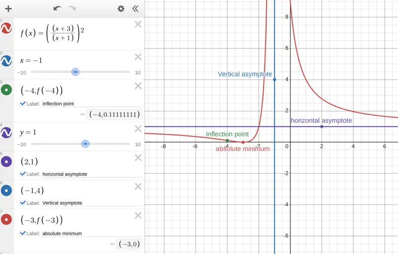
Figure: Graph of function
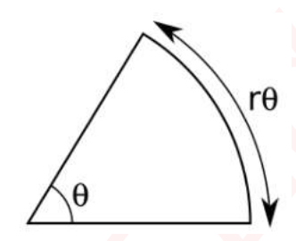
Hint: The area of a sector of angle radians in a circle of radius is , and the arc length of this sector is .
Exercise Tags
Tag:
Use the tag filtering feature on the course homepage to find all exercises with this tag.
Prerequisites for this Exercise
No prerequisite skills selected yet.
Unlock Premium Content
Get instant access to detailed walkthroughs, step-by-step explanations, and exclusive learning materials.
You want to maximize the area of a pizza slice, given that the perimeter of the slice is 60 cm. The perimeter consists of two straight sides (the radii) and the curved side (the arc of the circle).
Let:
- be the radius of the pizza slice.
- be the central angle of the pizza slice in radians.
The perimeter of the pizza slice is given by the sum of the two straight sides (each of length ) and the length of the arc:
You are told that the perimeter is 60 cm, so:
The area of the pizza slice is given by the formula for the area of a sector:
From the perimeter equation , solve for :
We now have in terms of , which we will substitute into the area formula to express the area as a function of .
Substitute into the area equation:
Simplify the expression:
So, the area function in terms of is:
To maximize the area, we need to take the derivative of with respect to and set it equal to zero. The derivative is:
Set to find the critical points:
Solving for :
To confirm that gives a maximum, take the second derivative of :
Since , which is negative, the function is concave down at , confirming that this is a maximum.
Because the second derivative is negative, this shows that the area is maximized at .
The radius that maximizes the area of the pizza slice is:
Unlock Premium Content
Get instant access to detailed solutions, step-by-step explanations, and exclusive learning materials.
Exercise Tags
Tag:
Use the tag filtering feature on the course homepage to find all exercises with this tag.
Prerequisites for this Exercise
No prerequisite skills selected yet.
Unlock Premium Content
Get instant access to detailed walkthroughs, step-by-step explanations, and exclusive learning materials.
Unlock Premium Content
Get instant access to detailed solutions, step-by-step explanations, and exclusive learning materials.
Sub-questions:
solution.
Exercise Tags
Tag:
Use the tag filtering feature on the course homepage to find all exercises with this tag.
Prerequisites for this Exercise
No prerequisite skills selected yet.
Unlock Premium Content
Get instant access to detailed walkthroughs, step-by-step explanations, and exclusive learning materials.
The Intermediate Value Theorem (IVT) states that if a continuous function takes opposite signs at two points and (i.e., ), then there exists at least one value in the interval such that .
We will use this theorem to show that the equation has at least one solution.
For the IVT to apply, the function must be continuous and change signs between two points.
Rearrange the equation to one side:
We are looking for values and such that , indicating the function changes sign over the interval.
We will evaluate at and exactly, without approximations.
1. **For **:
Thus, .
2. **For **:
Using exact values:
So:
Now we compare the signs of and :
- is positive.
- .
Since and , the expression is negative.
Therefore, , meaning the function changes sign over the interval . By the Intermediate Value Theorem, there is at least one value in the interval such that:
Thus, the equation has at least one solution in the interval:
The IVT guarantees a root in the interval where the function changes signs, even if the exact root is not known.
Unlock Premium Content
Get instant access to detailed solutions, step-by-step explanations, and exclusive learning materials.
Exercise Tags
Tag:
Use the tag filtering feature on the course homepage to find all exercises with this tag.
Prerequisites for this Exercise
No prerequisite skills selected yet.
Unlock Premium Content
Get instant access to detailed walkthroughs, step-by-step explanations, and exclusive learning materials.
The Mean Value Theorem (MVT) states that if a function is continuous on a closed interval and differentiable on the open interval , then there exists at least one point in the interval such that:
To show that the given equation has at most one solution, we need to prove that the function derived from this equation is either strictly increasing or strictly decreasing. This ensures the function cannot cross the x-axis more than once.
The MVT helps confirm that if the derivative does not equal zero, the function is strictly increasing or decreasing.
We rearrange the given equation into the form:
Now, differentiate to determine its behavior:
Applying standard derivative rules:
We now analyze the derivative to determine whether it is always positive, negative, or zero:
1. **The term ** is always positive for all , so is always negative.
2. **The term ** oscillates between and . Thus, oscillates between and .
3. **The constant term ** is always negative.
Together:
Since for all , the oscillations of cannot make the derivative positive. Thus:
Since for all , the function is strictly decreasing. A strictly decreasing function can intersect the x-axis at most once, meaning the equation has at most one solution.
A strictly decreasing function implies that the function values are unique for each , ensuring no more than one solution exists.
Using the MVT, we conclude that the equation:
can have at most one solution.
This problem tests your ability to apply the Mean Value Theorem in an abstract setting. The goal is to help students recognize how derivative behavior determines whether a function is increasing or decreasing. The professor wants to ensure you understand that the uniqueness of solutions relies on whether the function’s derivative maintains a consistent sign.
Unlock Premium Content
Get instant access to detailed solutions, step-by-step explanations, and exclusive learning materials.
Given:
The derivative is:
Since is always negative and is also always negative, we conclude that:
Because for all , the function is strictly decreasing, so the equation has at most one solution: