Practice Final #5
Full CourseExam Settings
Short Answer Questions
Short AnswerExercise Tags
Tag:
Use the tag filtering feature on the course homepage to find all exercises with this tag.
Prerequisites for this Exercise
No prerequisite skills selected yet.
We need to compute the indefinite integral . The integrand involves a function inside a square root, , and its derivative (up to a constant factor), , is present as the term outside the square root. This structure suggests using integration by substitution (u-substitution).
Let be the inner function:
Now, find the differential by differentiating with respect to :
Rearrange to solve for :
Notice that our integral has , not . We can solve the differential equation for : . This allows us to substitute perfectly.
Rewrite the original integral using and .
Substitute and :
Now integrate using the power rule for integration: (for ).
Here, , so .
Don't forget the constant of integration, , when computing indefinite integrals!
Replace with its expression in terms of , which is .
Exercise Tags
Tag:
Use the tag filtering feature on the course homepage to find all exercises with this tag.
Prerequisites for this Exercise
No prerequisite skills selected yet.
We need to evaluate the definite integral of the function over the interval . This involves finding the antiderivative of and evaluating it at the upper and lower limits of integration using the Fundamental Theorem of Calculus, Part 2.
We need to find a function such that its derivative is equal to .
Remember the basic derivative rules for trigonometric functions: the derivative of is . Therefore, the antiderivative of is , because the derivative of is .
So, the antiderivative is .
The Fundamental Theorem of Calculus, Part 2, states that if is an antiderivative of , then:
In our case, , , , and .
Now we need to evaluate at the upper limit and the lower limit .
Recall the values of cosine at these key angles: and .
Substitute these values into the expression:
The value of the definite integral is 1.
Exercise Tags
Tag:
Use the tag filtering feature on the course homepage to find all exercises with this tag.
Prerequisites for this Exercise
No prerequisite skills selected yet.
We already found that:
Setting the derivative equal to zero:
Since the denominator is never zero on our interval, we have:
This gives us or . Since is outside our interval , we only consider .
We need to check the function value at , , and .
At :
At :
At :
Comparing all three values:
-
-
-
The maximum value is which occurs at .
For rational functions, the behavior may be very different on different intervals. Always check all critical points within the interval AND both endpoints!
Exercise Tags
Tag:
Use the tag filtering feature on the course homepage to find all exercises with this tag.
Prerequisites for this Exercise
No prerequisite skills selected yet.
We already found the derivative of this function in our previous question:
To find critical points, we set this equal to zero:
Since the denominator cannot be zero on our interval (as when ), we only need:
So or are our critical points.
Our interval is , and we found one critical point at which is within this interval.
Extreme Value Theorem tells us that the maximum must occur either at a critical point within the interval or at an endpoint.
We need to evaluate the function at , , and .
When finding extreme values on a closed interval, always check both the critical points inside the interval AND the endpoint values!
Comparing all three values:
-
-
-
The maximum value is which occurs at .
Exercise Tags
Tag:
Use the tag filtering feature on the course homepage to find all exercises with this tag.
Prerequisites for this Exercise
No prerequisite skills selected yet.
We have a function with two terms:
1.
2.
We'll need to find the derivative of each term using the product rule, then evaluate at .
For the first term, , we use the product rule:
For the second term, , we use the product rule again:
When differentiating terms with , remember that . The coefficient comes out front!
The complete derivative is:
Now we evaluate at :
Therefore:
Mcq Questions
MCQat the point .
What is ? (2.5 points)
(A)
(B)
(C)
(D)
(E)
Exercise Tags
Tag:
Use the tag filtering feature on the course homepage to find all exercises with this tag.
Prerequisites for this Exercise
No prerequisite skills selected yet.
Unlock Premium Content
Get instant access to detailed walkthroughs, step-by-step explanations, and exclusive learning materials.
We already know the derivative is:
Evaluating it at :
So:
Thus, the point is:
The equation of the line is:
Substitute and :
Simplify:
Solve for :
The -intercept is:
Thus, the correct answer is:
Unlock Premium Content
Get instant access to detailed solutions, step-by-step explanations, and exclusive learning materials.
at the point .
What is ? (2.5 points)
(A)
(B)
(C)
(D)
(E)
Exercise Tags
Tag:
Use the tag filtering feature on the course homepage to find all exercises with this tag.
Prerequisites for this Exercise
No prerequisite skills selected yet.
Unlock Premium Content
Get instant access to detailed walkthroughs, step-by-step explanations, and exclusive learning materials.
We use the quotient rule to differentiate:
The quotient rule states:
where and .
Now:
Simplify:
Thus:
The slope of the tangent line at is:
Thus, the correct answer is:
Unlock Premium Content
Get instant access to detailed solutions, step-by-step explanations, and exclusive learning materials.
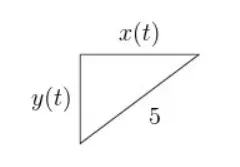
Figure: right triangle
What is the ratio when ? Assume that is non-zero.
(A)
(B)
(C)
(D)
(E)
Exercise Tags
Tag:
Use the tag filtering feature on the course homepage to find all exercises with this tag.
Prerequisites for this Exercise
No prerequisite skills selected yet.
Unlock Premium Content
Get instant access to detailed walkthroughs, step-by-step explanations, and exclusive learning materials.
We are given a right-angled triangle with a hypotenuse that is always 5 cm long. The sides are , , and the hypotenuse is . So the Pythagorean theorem gives:
Simplify:
Divide both sides by :
Thus:
Using the Pythagorean theorem:
The ratio when is:
Thus, the correct answer is:
Unlock Premium Content
Get instant access to detailed solutions, step-by-step explanations, and exclusive learning materials.
(A)
(B)
(C)
(D)
(E)
Exercise Tags
Tag:
Use the tag filtering feature on the course homepage to find all exercises with this tag.
Prerequisites for this Exercise
No prerequisite skills selected yet.
Unlock Premium Content
Get instant access to detailed walkthroughs, step-by-step explanations, and exclusive learning materials.
We recognize that the integral of is the well-known inverse tangent function:
The integral of is:
Now we combine the two integrals:
where is the most general constant of integration.
Thus, the most general antiderivative is:
The correct answer is:
Unlock Premium Content
Get instant access to detailed solutions, step-by-step explanations, and exclusive learning materials.
(A)
(B)
(C)
(D)
(E)
Exercise Tags
Tag:
Use the tag filtering feature on the course homepage to find all exercises with this tag.
Prerequisites for this Exercise
No prerequisite skills selected yet.
Unlock Premium Content
Get instant access to detailed walkthroughs, step-by-step explanations, and exclusive learning materials.
We are trying to evaluate:
We can rewrite this as:
By splitting it like this, we can analyze each part separately, making it easier to solve.
1. **Evaluate** :
This is a standard limit that often appears in exams.
[Remember this limit:
They love to test this! It shows that and are almost identical for small values of .]
2. **Evaluate** :
For small , the function behaves similarly to .
[This limit is another must-know:
This shows that for small , the numerator and denominator act like the same function.]
3. **Evaluate** :
This tells us that the function grows without bound as approaches 0 from the positive side.
Using the property that:
**(only if all limits are finite or one limit goes to infinity without any undefined behavior like )**, we get:
Since the multiplication involves finite values and one , the result is:
This approach works here because each limit we evaluated behaves predictably and does not lead to an undefined form like . Therefore, we can confidently multiply the individual limits.
In this tough question they are testing your knowledge of the these two limits:
and
. As long as you know those limits then you'll have no problem with this question.
The reciprocal of each limit is also 1:
These limits show that and behave almost exactly like when is close to 0. Knowing these will help you solve many tricky limits that appear in calculus exams!
You can also therefore mix these terms:
Both and behave like when is close to 0, so this limit simplifies to:
This is another handy limit to keep in mind for calculus exams!
Unlock Premium Content
Get instant access to detailed solutions, step-by-step explanations, and exclusive learning materials.
Long Answer Questions
Long AnswerExercise Tags
Tag:
Use the tag filtering feature on the course homepage to find all exercises with this tag.
Prerequisites for this Exercise
No prerequisite skills selected yet.
The integral is .
The denominator contains . This looks similar to the form , which appears in the derivative of arcsin and arccos.
Let's try to match the form . We can write and . So, the term inside the square root is .
This suggests choosing and making the substitution .
Let's check the derivative: . The numerator of the integrand is , which is proportional to this derivative.
This confirms that u-substitution with is a good strategy, aiming for the arcsine integral form.
Let .
Find the differential :
Our integral contains the term . Solve for it from the differential:
Now substitute (so ) and into the integral:
The integral is now in a standard form.
Recall the integration rule involving arcsine: .
In our case, . Applying this rule:
Replace with its expression in terms of , which is .
The indefinite integral is . This result is concise enough for the KaTeX `\boxed{}`.
Determine where the function is increasing and decreasing.
Determine where the function is concave up and concave down.
Exercise Tags
Tag:
Use the tag filtering feature on the course homepage to find all exercises with this tag.
Prerequisites for this Exercise
No prerequisite skills selected yet.
Let's work with the function:
To find the first derivative, I'll use the product rule:
Where:
-
-
First, I'll find :
Now applying the product rule:
For the second derivative, I'll apply the product rule again to
Where:
-
-
First, I'll find :
Now applying the product rule:
A function is increasing when and decreasing when .
Let's find where :
Since for all , we need to solve:
This gives us or
When analyzing where a function is increasing or decreasing, focus on where the first derivative changes sign.
Testing regions:
- For : and , so , meaning
- For : and , so , meaning
- For : and , so , meaning
Therefore:
- is increasing for
- is decreasing for
- is increasing for
A function is concave up when and concave down when .
From our second derivative:
Since for all , we need to solve :
Testing regions:
- For : , so
- For : , so
- For : , so
Therefore:
- is concave up for
- is concave down for
- is concave up for
Classify each such point as a local minimum, a local maximum or some other kind of critical point.
Exercise Tags
Tag:
Use the tag filtering feature on the course homepage to find all exercises with this tag.
Prerequisites for this Exercise
No prerequisite skills selected yet.
Let's work with the function: in the interval .
To find critical points, I need to take the derivative and set it equal to zero.
When differentiating products, remember that the derivative of follows the product rule:
This equation equals zero when either:
- , which gives
- , which gives where is an integer
In our interval , when:
So our critical points are:
-
-
-
-
To classify, I'll use the second derivative test.
Now I'll evaluate at each critical point:
At :
Since , this is a local minimum.
At :
Since , this is a local maximum.
At :
Since , this is a local minimum.
At :
Since , this is a local maximum.
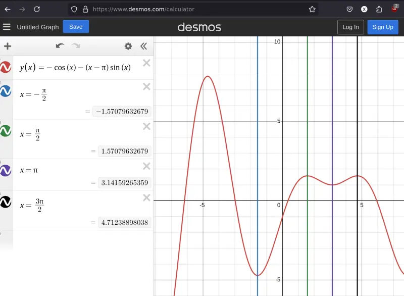
Figure: solution
Multi Part Questions
Multi-PartExercise Tags
Tag:
Use the tag filtering feature on the course homepage to find all exercises with this tag.
Prerequisites for this Exercise
No prerequisite skills selected yet.
Unlock Premium Content
Get instant access to detailed walkthroughs, step-by-step explanations, and exclusive learning materials.
Unlock Premium Content
Get instant access to detailed solutions, step-by-step explanations, and exclusive learning materials.
Sub-questions:
Exercise Tags
Tag:
Use the tag filtering feature on the course homepage to find all exercises with this tag.
Prerequisites for this Exercise
No prerequisite skills selected yet.
Unlock Premium Content
Get instant access to detailed walkthroughs, step-by-step explanations, and exclusive learning materials.
The function is:
Both (a polynomial) and (an exponential function) are continuous for all . Therefore, the sum of these functions is continuous everywhere.
**Step 1: Find the First Derivative **
Using the product rule:
Applying the product rule to the first term:
Simplify:
Factor out :
**Step 2: Solve for Critical Points**
Since for all real , solve:
**Critical Points:**
**Step 1: Find the Second Derivative **
Using the product rule on the first derivative:
Differentiate:
The derivative of is:
Now substitute:
Simplify:
Factor out :
**Step 2: Solve for Inflection Points**
Since , solve:
This gives two cases:
1. .
2. .
Solve the second equation:
**Inflection Points:**
---
- **Discontinuities:** None.
- **Critical Points:** .
- **Inflection Points:**
Unlock Premium Content
Get instant access to detailed solutions, step-by-step explanations, and exclusive learning materials.
- **Critical Points:** .
- **Inflection Points:**
Exercise Tags
Tag:
Use the tag filtering feature on the course homepage to find all exercises with this tag.
Prerequisites for this Exercise
No prerequisite skills selected yet.
Unlock Premium Content
Get instant access to detailed walkthroughs, step-by-step explanations, and exclusive learning materials.
We are analyzing the function:
Horizontal asymptotes occur when the function approaches a constant value as or .
Since very quickly as , the first term also approaches 0:
Now, check the behavior as :
Similarly, as , the term also approaches 0:
**Horizontal Asymptote:**
---
A **vertical asymptote** occurs when the function becomes arbitrarily large (positively or negatively) as approaches a specific finite value. More formally, a function has a vertical asymptote at if:
Such asymptotic behavior typically arises when:
- The function has a division by zero, such as in .
- There are logarithmic terms, like , which decrease without bound as the input approaches a critical point.
- Or other forms of singularities that force the function to grow indefinitely large.
---
### Step 2.1: Analyze the Function
We now analyze the structure of the given function. It contains:
- A linear term .
- An exponential decay term , which approaches rapidly as or .
We are checking if there are any values of for which the function becomes undefined or grows without bound.
---
### Step 2.2: Look for Potential Asymptotes
Let’s examine the key term :
1. **Behavior as :**
- As increases, decays very quickly to . This decay outpaces the growth of the linear term .
- Therefore, the product as .
2. **Behavior as :**
- Similarly, as becomes increasingly negative, the term also approaches , and the product again approaches .
Because the function remains finite in both directions and there are no divisions by zero or undefined values for any finite , the function is continuous across all real numbers.
---
**Conclusion: There are no vertical asymptotes.** The function is well-defined and continuous everywhere for , with no points where the function becomes arbitrarily large or undefined.
- **Horizontal Asymptote:** .
- **Vertical Asymptotes:** None.
Unlock Premium Content
Get instant access to detailed solutions, step-by-step explanations, and exclusive learning materials.
- **Vertical Asymptotes:** None.
Exercise Tags
Tag:
Use the tag filtering feature on the course homepage to find all exercises with this tag.
Prerequisites for this Exercise
No prerequisite skills selected yet.
Unlock Premium Content
Get instant access to detailed walkthroughs, step-by-step explanations, and exclusive learning materials.

Figure 1: all critical points, inflection points, and asymptotes
Unlock Premium Content
Get instant access to detailed solutions, step-by-step explanations, and exclusive learning materials.
Figure 1: all critical points, inflection points, and asymptotes
Exercise Tags
Tag:
Use the tag filtering feature on the course homepage to find all exercises with this tag.
Prerequisites for this Exercise
No prerequisite skills selected yet.
Unlock Premium Content
Get instant access to detailed walkthroughs, step-by-step explanations, and exclusive learning materials.
Unlock Premium Content
Get instant access to detailed solutions, step-by-step explanations, and exclusive learning materials.
Sub-questions:
Exercise Tags
Tag:
Use the tag filtering feature on the course homepage to find all exercises with this tag.
Prerequisites for this Exercise
No prerequisite skills selected yet.
Unlock Premium Content
Get instant access to detailed walkthroughs, step-by-step explanations, and exclusive learning materials.
The function given is:
This is a rational function, meaning it is a fraction with a polynomial in the numerator and denominator. The square does not affect the domain restrictions, so we can focus on finding when the denominator equals zero.
The denominator is , and the function is undefined when the denominator is zero because division by zero is not allowed.
So, we set the denominator equal to zero:
Solving for :
This means the function is undefined at .
The domain of is all real numbers except . In interval notation, the domain is:
Unlock Premium Content
Get instant access to detailed solutions, step-by-step explanations, and exclusive learning materials.
Exercise Tags
Tag:
Use the tag filtering feature on the course homepage to find all exercises with this tag.
Prerequisites for this Exercise
No prerequisite skills selected yet.
Unlock Premium Content
Get instant access to detailed walkthroughs, step-by-step explanations, and exclusive learning materials.
Critical numbers occur where the derivative of a function is either zero or undefined. However, these points must be within the domain of the original function to be considered valid critical numbers.
Given:
To differentiate, we apply the chain rule and quotient rule. Let:
Using the chain rule:
Now, we apply the quotient rule to find . For , the quotient rule states:
For and :
Substitute these into the quotient rule:
Simplify:
Now, substitute into the derivative of :
Simplify:
To find the critical numbers, we need to determine where the derivative is zero or undefined.
- **When :**
The fraction equals zero when the numerator is zero:
- **When is undefined:**
The derivative is undefined when the denominator is zero:
However, itself is undefined at , so this value is not a valid critical number.
Since is outside the domain of the function, the only valid critical number is:
This problem tests your ability to find critical numbers by correctly applying the chain rule and quotient rule. A key takeaway is that critical numbers must be within the function’s domain—points where the derivative is undefined but are outside the domain are not considered valid. The professor wants you to understand how to handle both cases where the derivative is zero and where it is undefined while also considering the original function’s domain.
Unlock Premium Content
Get instant access to detailed solutions, step-by-step explanations, and exclusive learning materials.
Exercise Tags
Tag:
Use the tag filtering feature on the course homepage to find all exercises with this tag.
Prerequisites for this Exercise
No prerequisite skills selected yet.
Unlock Premium Content
Get instant access to detailed walkthroughs, step-by-step explanations, and exclusive learning materials.
A point of inflection occurs where the concavity of the function changes, which happens when the second derivative, , changes sign. To find potential points of inflection, we need to:
1. Find the second derivative .
2. Determine where or undefined.
3. Check if the concavity changes at those points.
A point of inflection occurs only if the concavity changes from concave up to concave down (or vice versa).
We already know that:
Now, let's differentiate to find using the quotient rule. The quotient rule for is:
For , we have:
-
-
Substitute these into the quotient rule:
Simplify the numerator:
Factor out from the numerator:
Simplify further:
Now, we set and solve for :
The fraction is zero when the numerator is zero, so:
Also, is undefined when the denominator is zero, which happens when:
However, is not in the domain of the function (as found in part (a)).
Points where is undefined may still be points of inflection if the concavity changes across those points, but only if they lie in the domain.
To confirm that is a point of inflection, we check the sign of on either side of .
- For (e.g., ), , so the function is concave down.
- For (e.g., ), , so the function is concave up.
Since the concavity changes from concave down to concave up, is a point of inflection.
The possible point of inflection is:
Unlock Premium Content
Get instant access to detailed solutions, step-by-step explanations, and exclusive learning materials.
Exercise Tags
Tag:
Use the tag filtering feature on the course homepage to find all exercises with this tag.
Prerequisites for this Exercise
No prerequisite skills selected yet.
Unlock Premium Content
Get instant access to detailed walkthroughs, step-by-step explanations, and exclusive learning materials.
Horizontal asymptotes occur when the function approaches a constant value as tends to infinity or negative infinity. To find horizontal asymptotes, we calculate the limits of the function as and .
The given function is:
We'll examine the limits as and .
Remember, horizontal asymptotes describe the behavior of the function as tends to very large positive or negative values.
First, we calculate the limit of as :
Divide both the numerator and the denominator by to simplify the expression:
As , both and approach zero, so the expression simplifies to:
Thus, the horizontal asymptote as is .
Next, we calculate the limit of as :
Again, divide the numerator and the denominator by :
As , both and approach zero, so the expression simplifies to:
Thus, the horizontal asymptote as is also .
Since both limits as and yield the same value, the function has a horizontal asymptote at:
Horizontal asymptotes tell us the behavior of the function as approaches extreme values.
Unlock Premium Content
Get instant access to detailed solutions, step-by-step explanations, and exclusive learning materials.
Exercise Tags
Tag:
Use the tag filtering feature on the course homepage to find all exercises with this tag.
Prerequisites for this Exercise
No prerequisite skills selected yet.
Unlock Premium Content
Get instant access to detailed walkthroughs, step-by-step explanations, and exclusive learning materials.
A vertical asymptote occurs where the function approaches infinity (or negative infinity) as approaches a certain value. Vertical asymptotes are typically found by identifying values of that make the denominator of a rational function equal to zero, causing the function to be undefined.
The given function is:
For this function, we look at when the denominator is zero because division by zero creates vertical asymptotes.
Vertical asymptotes occur where the denominator of a rational function is zero and the function becomes undefined.
Set the denominator equal to zero:
Solving for :
Thus, the function is undefined at . This means there is a potential vertical asymptote at .
To confirm that is a vertical asymptote, we analyze the behavior of the function as approaches from both the left and the right:
1. **As (approaching from the right):**
When approaches from values greater than , is positive but very small. Thus, becomes very large, and squaring it makes approach .
2. **As (approaching from the left):**
When approaches from values smaller than , is negative but very small. In this case, becomes very large but negative, and squaring it still makes approach .
In both cases, as approaches , the function tends to infinity, confirming that is a vertical asymptote.
The vertical asymptote occurs at:
Remember, vertical asymptotes occur where the function becomes undefined and approaches or .
Unlock Premium Content
Get instant access to detailed solutions, step-by-step explanations, and exclusive learning materials.
Exercise Tags
Tag:
Use the tag filtering feature on the course homepage to find all exercises with this tag.
Prerequisites for this Exercise
No prerequisite skills selected yet.
Unlock Premium Content
Get instant access to detailed walkthroughs, step-by-step explanations, and exclusive learning materials.
From the previous parts, we know the following:
- The **critical number** of is (from part (b)).
- The **point of inflection** is at (from part (c)).
- There is a **vertical asymptote** at (from part (e)).
- The **domain** of the function is (from part (a)).
We will use these points to create a table of signs for and .
We already found . Now we check the sign of in each interval determined by the critical point and the vertical asymptote .
| Interval | Test Point | Sign of | Behavior of |
|---|---|---|---|
| Positive | Increasing | ||
| Negative | Decreasing | ||
| Negative | Decreasing |
So, the function is increasing on and decreasing on .
We already found . Now we check the sign of in each interval determined by the point of inflection and the vertical asymptote .
| Interval | Test Point | Sign of | Concavity of |
|---|---|---|---|
| Concave Down | |||
| Concave Up | |||
| Concave Up |
So, the function is concave down on and concave up on .
- **Increasing**:
- **Decreasing**:
- **Concave Down**:
- **Concave Up**:
Remember, increasing/decreasing behavior is determined by the sign of , and concavity is determined by the sign of .
Unlock Premium Content
Get instant access to detailed solutions, step-by-step explanations, and exclusive learning materials.
| Interval | Test Point | Sign of | Behavior of |
|---|---|---|---|
| Positive | Increasing | ||
| Negative | Decreasing | ||
| Negative | Decreasing |
| Interval | Test Point | Sign of | Concavity of |
|---|---|---|---|
| Concave Down | |||
| Concave Up | |||
| Concave Up |
Exercise Tags
Tag:
Use the tag filtering feature on the course homepage to find all exercises with this tag.
Prerequisites for this Exercise
No prerequisite skills selected yet.
Unlock Premium Content
Get instant access to detailed walkthroughs, step-by-step explanations, and exclusive learning materials.
Unlock Premium Content
Get instant access to detailed solutions, step-by-step explanations, and exclusive learning materials.
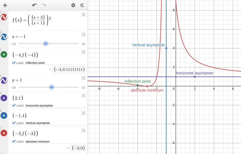
Figure: Graph of function